2 Improving Transparency
The most recent empirical evidence supporting the idea that regular use of digital technologies by teenagers negatively impacts their psychological well-being is largely based on secondary analyses of large-scale social datasets. Though these datasets provide a valuable resource for highly powered investigations, their many variables and observations are often explored with an analytic flexibility that marks small effects as statistically significant, thereby leading to potential false positives and conflicting results. Here I address these methodological challenges by applying Specification Curve Analysis across three large-scale social datasets (ntot = 355,358) to rigorously examine correlational evidence for digital technology affecting adolescents. The association I find between digital technology use and adolescent well-being is negative but small, explaining at most 0.4% of the variation in well-being. Taking the broader context of the data into account suggests that these effects are probably too small to warrant policy change.
2.1 Introduction
The idea that digital devices and the internet have an enduring influence on how humans develop, socialize, and thrive is a compelling one (Bell, Bishop, and Przybylski 2015). As the time young people spend online has doubled in the past decade (Ofcom 2019), the debate about whether this shift negatively impacts children and adolescents is becoming increasingly heated (Steers 2016). A number of professional and governmental organizations have therefore called for more research into digital screen time (House of Commons Science and Technology Select Committee 2019; British Youth Council 2017), which has led to household panel surveys (Johnston et al. 2016; Kann et al. 2016) and large-scale social datasets adding measures of digital technology use to those already assessing psychological well-being (University of London 2017). Unfortunately, findings derived from the cross-sectional analysis of these datasets are conflicting; in some cases negative associations between digital technology use and well-being are found (Etchells et al. 2016; Twenge et al. 2017), often receiving much attention even when correlations are small. Yet other results are mixed (Parkes et al. 2013) or contest previously found negative effects when re-analysing identical data (Ferguson 2018). A high-quality pre-registered analysis of UK adolescents found that moderate digital engagement does not correlate with well-being, but very high levels of usage possibly have small negative associations (Ferguson 2017; Przybylski and Weinstein 2017).
There are at least three reasons why the inferences behavioural scientists draw from large-scale datasets might produce divergent findings. First, these datasets are mostly collected in collaboration with multidisciplinary research councils and are characterized by a battery of items meant to be completed by postal survey, face-to-face or telephone interview (Johnston et al. 2016; Kann et al. 2016; University of London 2017). Though research councils engage in public consultations (National Health Service 2016), the pre-tested or validated scales common in clinical, social or personality psychology are often abbreviated or altered to reduce participant burden (U.S. Department of Health and Human Services, Health Resources and Services Administration and Bureau 2014; Livingstone et al. 2011). Scientists wishing to make inferences about digital technology’s effects using these data need to take numerous decisions about how to analyse, combine and interpret the measures. Taking advantage of these valuable datasets is therefore fraught with many subjective analytical decisions, which can lead to high numbers of researcher degrees of freedom (Silberzahn et al. 2018). With nearly all decisions taken after the data are known, they are not apparent to those reading the published paper highlighting only the final analytical pathway (Gelman and Loken 2014; Simmons, Nelson, and Simonsohn 2011).
The second possible explanation for conflicting patterns of effects found in large-scale datasets is rooted in the scale of the data analysed. Compared to the laboratory- and community-based samples typical of behavioural research (mostly < 1,000, Marszalek et al. 2011), large-scale social datasets feature high numbers of participant observations (ranging from n = 5,000 to n = 5,000,000, Johnston et al. 2016; Kann et al. 2016; University of London 2017). This means very small covariations (e.g. r’s < .01) between self-report items will result in compelling evidence for rejecting the null hypothesis at levels typically interpreted as statistically significant by behavioural scientists (i.e. p’s < .05). As minute correlations are arguably omnipresent in self-report data (Meehl 1990a, 1990b; Orben and Lakens 2019), such correlations are therefore more often labelled statistically significant.
Thirdly, it is important to note that most datasets are cross-sectional and therefore only provide correlational evidence, making it difficult to pinpoint causes and effects (see Chapter 4 for more detail). Thus, large-scale datasets are simultaneously attractive and problematic for researchers, peer reviewers and the public. They are a resource for testing behavioural theories at scale but are, at the same time, inherently susceptive to false positives and significant-but-minute effects using the levels traditionally employed in psychology.
Given that digital technology’s impact on child well-being is a topic of widespread scientific debate among those studying human behaviour (Bell, Bishop, and Przybylski 2015) and has real-world implications (House of Commons Science and Technology Select Committee 2019), it is important for researchers to make the most of existing large-scale dataset investments. This makes it necessary to employ transparent and robust analytic practices, which recognize that the measures of digital technology use and well-being in large-scale datasets may not be well-matched to specific research questions. Further, behavioural scientists must be transparent about how the hundreds of variables and many thousands of observations can quickly branch out into gardens of forking paths with millions, and in some cases billions of analysis options (Gelman and Loken 2014). This risk is compounded by a reliance on statistical significance, i.e. using p < .05, to demarcate ‘true’ effects. Unfortunately, the large number of participants in these designs means small effects are easily publishable and, if positive, garner outsized press and policy attention (Ferguson 2018).
As large-scale secondary datasets are increasingly available freely online, it is not possible to convincingly document a scientist’s ignorance of the data before analysis (Chambers 2013; Munafò et al. 2017; van’t Veer and Giner-Sorolla 2016), making hypothesis preregistration untenable as a general solution to the problem of subjective analytical decisions. Specification Curve Analysis (SCA, Simonsohn, Simmons, and Nelson 2015) provides a promising alternative (see 2.2.4 for further explanation). SCA is a tool for mapping the sum of theory-driven analytic decisions that could have been justifiably taken when analysing quantitative data. Researchers demarcate every possible analytical pathway and then calculate the results of each one. Instead of reporting a handful of analyses in their paper, they report all results of all theoretically defensible analyses. This approach has been published in the previous literature (Simonsohn, Simmons, and Nelson 2015; Rohrer, Egloff, and Schmukle 2017).
Because of the substantial disagreements within the literature, the extent to which adolescents’ screen-time may actually be impacting their psychological well-being remains unclear. The present chapter addresses this gap in our understanding by relying on large-scale data paired with a conservative analytic approach to provide a more transparent and clearly contextualized test of the association between screen use and well-being.
To this end, three large-scale exemplar datasets (Monitoring the Future, the Youth Risk and Behaviour Survey and the Millennium Cohort Study) from the US and the UK were selected to highlight the particular strengths and weaknesses of drawing general inferences from large-scale social data and how they can be reconceptualised by SCA (Johnston et al. 2016; Kann et al. 2016; University of London 2017). Further, I tackle the problem of significant-but-minimal effects in large-scale social data by using the abundance of questions in each dataset to compute comparison specifications; I directly compare the effects of digital technology to the effects of other activities on psychological well-being (e.g. sleep, eating breakfast, illicit drug use), using extant literatures and psychological theory as a guide. This allows me to simultaneously examine the impact of adolescent technology use against real-world benchmarks while modelling and accounting for analytic flexibility.
2.2 Methods
2.2.1 Datasets and Participants
This chapter’s analysis pipeline spans three nationally-representative datasets from the US and the UK (Johnston et al. 2016; Kann et al. 2016; University of London 2017), encompassing a total of 355,358, predominately twelve- to eighteen-year-old, adolescents surveyed between the years of 2007 and 2016. These datasets were selected because they feature measures of adolescents’ psychological well-being, digital technology use, and have been the focus of secondary data analysis to study digital technology effects [Parkes et al. (2013); Twenge et al. (2017); Twenge, Martin, and Campbell (2018); Kelly2019]. Furthermore, the American datasets were analysed in a paper that I evaluated in a blogpost at publication, and which initially motivated me to do this research (Twenge et al. 2017; Orben 2017).
Two datasets are based on samples collected in the United States. The first, the Youth Risk and Behaviour Survey (YRBS, Kann et al. 2016) launched in 1990, is a biennial survey of adolescents that reflects a nationally-representative sample of students attending secondary schools in the US (years 9-12). The resulting sample from the YRBS was collected from 2007 to 2015 and included 37,402 girls and 37,412 boys, ranging in age from “12 years or younger” to “18 years or older” ( = 16, s.d. = 1.24). The second US dataset, Monitoring the Future (MTF, Johnston et al. 2016), launched in 1975 and is an annual nationally-representative survey of approximately 50,000 American adolescents in Grades 8, 10 and 12. While the survey includes adolescents in Grade 12, many of the key items of interest cannot be correlated in their survey, and therefore their data were not included in my analysis. The resulting sample from the MTF was collected from 2008 to 2016, and included 136,190 girls and 132,482 boys, though the exact age of individual respondents was removed from the dataset by study coordinators during anonymization.
The UK dataset under analysis was the Millennium Cohort Study (MCS, University of London 2017), a prospective study collected in the UK; it follows a specific cohort of children born between September 2000 and January 2001. These data were not previously analysed by the studies that motivated this work, but were added because I see these data as particularly high in quality. This is mostly due to its inclusion of pre-tested measures and extensive documentation, highlighting good data collection and project management practices. The dataset has an over-representation of minority groups and disadvantaged areas due to clustered stratified sampling. Data in this sample is provided by caregivers as well as adolescent participants. In my analysis, I only include data from the primary caregivers and adolescent respondents. The sample under analysis from the MCS was comprised of 5,926 girls and 5,946 boys who ranged in age from 13 to 15 ( = 13.77, s.d. = .45) and 10,605 primary caregivers.
While the omnibus sample of adolescents is 355,358 teenagers in total, it is important to note that the sample sizes of the analyses are often smaller, in some cases by an order of magnitude or more. This is due to missing values, but also because in questionnaires like MTF teenagers only answered a subset of questions. More information about what questions were asked together in MTF can be found on the Open Science Framework (OSF; Table 1, http://dx.doi.org/10.17605/OSF.IO/87QGM)
2.2.2 Ethical Review
Ethical review and approval for data collection for YRBS was conducted and granted by the CDC Institutional Review Board. The University of Michigan Institutional Review Board oversees MTF. Ethical review and approval for the MCS is monitored by the UK National Health Service, London, Northern, Yorkshire and South-West Research Ethics Committees.
2.2.3 Measures
This study focuses on measures of both digital technology use and psychological well-being. Prior to performing the analysis, all three datasets were reviewed, noting the variables of theoretical interest in each with respect to human behaviour and effects of technology engagement. Some questions have been modified with successive waves of data collection. In all cases these changes are relatively minor and are noted in the OSF repository (Table 2, http://dx.doi.org/10.17605/OSF.IO/87QGM). In my ongoing analyses I use the questionnaires in many different constellations and therefore refrain from including reliability measurements.
2.2.3.1 Criterion Variables: Adolescent Well-Being
All datasets contained a wide range of different questions that concern the adolescents’ psychological well-being and functioning. I reversed select measures so that they are all in the same direction, with higher scores indicating higher well-being.
Adolescents were asked five items related to mental health and suicidal ideation in the YRBS. Three of the items were on a yes-no scale: “During the past 12 months did you ever:”, “feel so sad or hopeless almost every day for two weeks or more in a row that you stopped doing some usual activities”, “seriously consider attempting suicide”, “make a plan about how you would attempt suicide”. There was also one measure asking “During the 12 months, how many times did you actually attempt suicide?” (1 = “0 times” to 5 = “6 or more times”). I recoded this measure to 1 = 0 times and 0 = 1 or more times. Furthermore, there was one question about “if you attempted suicide during the past 12 months, did any attempts result in an injury, poisoning, or overdose that had to be treated by a doctor or nurse?”, (1 = “I did not attempt suicide during the past 12 months”“, 2 = "Yes"”, 3 = “No”). I recoded this measure so 1 = did not attempt suicide or did not need to be treated by doctor or nurse, 0 = needed to be treated by doctor or nurse.
In MTF, participants were asked one of two subsets of self-report questions. The first tranche of participants was asked thirteen questions about their mental health: twelve measures uniquely asked to this subset, and one measure completed by all participants in the survey. The twelve items asked only to this subset included a four-item depressive symptoms scale which studies state to be “similar to those on the Center for Epidemiologic Studies Depression Scale (Maslowsky, Schulenberg, and Zucker 2014): five-point scale (1 = “disagree” to 5 = “agree”), “Life often seems meaningless” (reverse coded), “I enjoy life as much as anyone”, “The future often seems hopeless” (reverse coded), “It feels good to be alive”. The study also included the Rosenberg Self-Esteem scale which was presented on a similar five-point scale (Maslowsky, Schulenberg, and Zucker 2014): “I take a positive attitude towards myself”, “Sometimes I think that I am no good at all” (reverse coded), “I feel I am a person of worth, on an equal plane with others”, “I am able to do things as well as most other people” and “I feel I do not have much to be proud of” (reverse coded). There were, furthermore, two additional negative self-esteem items added by the MTF survey administrators to ensure there were an equal amount of positively and negatively coded self-esteem items: “I feel that I can’t do anything right” (reverse coded), “I feel that my life is not very useful” (reverse coded). I do not include “Sometimes I am no good at all” as a measure in my SCA, as it could not be clearly attributed to a questionnaire. Participants of all subsets were additionally asked a single life satisfaction measure: “Taken all things together, how would you say things are these days – would you say you’re very happy (3, recoded to 2), pretty happy (2, recoded to 1) or not to happy these days (1, recoded to 0)?”
There are two kinds of psychological well-being indicators included in the MCS: (1) those filled out by the cohort members, and (2) those completed by their primary caregivers. To measure wellbeing, MCS participants were asked how they felt about “your school work”, “the way you look”, “your family”, “your friends”, “the school you go to”, “your life as a whole” (1 = completely happy, 7 = not at all happy, scale subsequently reversed). They were also asked five items from an abbreviated self-esteem measure (Robins, Hendin, and Trzesniewski 2001): “On the whole, I am satisfied with myself”, “I feel I have a number of good qualities”, “I am able to do things as well as most other people”, “I am a person of value”, “I feel good about myself” (1 = strongly agree to 4 = strongly disagree, scale subsequently reversed). Finally, they were asked twelve questions tapping subjective affective states and general mood (Angold et al. 1995): “For each question please select the answer which reflects how you have been feeling or acting in the past two weeks:”, “I felt miserable or unhappy”, “I didn’t enjoy anything at all”, “I felt so tired I just sat around and did nothing”, “I was very restless”, “I felt I was no good any more”, “I cried a lot”, “I found it hard to think properly or concentrate”, “I hated myself”, “I was a bad person”, “I felt lonely”, “I thought nobody really loved me”, “I thought I could never be as good as other kids” and “I did everything wrong” (1 = not true, 2 = sometimes, 3 = true, scale subsequently reversed).
Primary caregivers completed the Strengths and Difficulties Questionnaire (SDQ) (Goodman et al. 2000), a well-validated measure of psychosocial functioning, for each adolescent cohort member they took care of (Table 2.1). The SDQ has been used extensively in school, home, and clinical settings with adolescents from a wide range of social, ethnic, and national backgrounds (Desai, Chase-Lansdale, and Michael 1989). It includes 25 questions, five each about prosocial behaviour, hyperactivity or inattention, emotional symptoms, conduct problems and peer relationship problems.
| Question | Not True | Somewhat True | Certainly True |
|---|---|---|---|
| Considerate of other people’s feelings | |||
| Restless, overactive, cannot stay still for long | |||
| Often complains of headaches, stomach-aches or sickness | |||
| Shares readily with other children (treats, toys, pencils etc.) | |||
| Often has temper tantrums or hot tempers | |||
| Rather solitary, tends to play alone | |||
| Generally obedient, usually does what adults request | |||
| Many worries, often seems worried | |||
| Helpful if someone is hurt, upset or feeling ill | |||
| Constantly fidgeting or squirming | |||
| Has at least one good friend | |||
| Often fights with other children or bullies them | |||
| Often unhappy, down-hearted or tearful | |||
| Generally like by other children | |||
| Easily distracted, concentration wanders | |||
| Nervous or clingy in new situations, easily loses confidence | |||
| Kind to younger children | |||
| Often lies or cheats | |||
| Picked on or bullied by other children | |||
| Often volunteers to help others (parents, teachers, other children) | |||
| Thinks things out before acting | |||
| Steals from home, school or elsewhere | |||
| Gets on better with adults than with other children | |||
| Many fears, easily scared | |||
| Sees tasks through to the end, good attention span |
2.2.3.2 Explanatory variables: Adolescent Technology Use
The YRBS dataset included two seven-point technology use questions. One YRBS technology use question was about the use of electronic devices, “On an average school day, how many hours do you play video or computer games or use a computer for something that is not school work? (Count time spent on things such as Xbox, PlayStation, an iPad or other tablet, a smartphone, texting, YouTube, Instagram, Facebook or other social media)”, (1 = “I do not play video or computer games or use a computer for something that is not school work” to 7 = “5 or more hours per day”). The other question asked “on an average school day, how many hours do you watch TV?”, (1 = “I do not watch TV on an average school day” to 7 = “5 or more hours per day”).
The MTF asked a variety of technology use questions. As the questionnaire was split into six parts (with each participant only filling in one part), some questions were filled out by one subset of adolescents, while other questions were filled out by another. One subset answered questions about frequency of social media use and getting information about news from the internet (five-point scale): “How often do you do each of the following? Visit social networking websites (like Facebook)” and “How often do you use each of the following to get information about news and current events? The internet.”. Both questions were coded on a five-point scale (1 = never to 5 = almost every day). Furthermore, these participants were asked two seven-point questions about frequency of watching TV on the weekend and weekday: “How much TV do you estimate you watch on an average weekend/weekday?”, seven-point scale (1 = none to 7 = nine or more hours). Another group of MTF participants were asked seven hourly measures of technology use on a nine-point scale (1 = none to 9 = 40 hours or more). The questions asked about using the internet, playing electronic games, texting on a cell phone, calling on a cell phone, using social media, video chatting and using computers for school. There are, therefore, a total of eleven technology use measures that can be used when analysing the MTF dataset.
In the MCS, the participants were asked five questions concerning technology use. The MCS included four eight-point questions about hours per weekday spent “watching television programmes or films”, spent “playing electronic games on a computer or games systems”, “spent using the internet” at home and spent “on social networking or messaging sites or Apps on the internet” (1 = none to 8 = 7 hours or more). There was also one yes-no measure about whether participants own a computer: “do you have a computer … of your own?”.
2.2.3.3 Control variables
Mirroring previous studies analysing data from the MCS (University of London 2017), I included sociodemographic factors and maternal characteristics as control variables (i.e. covariates) in my analyses. These include mother’s ethnicity, education, employment and psychological distress (using the K6 Kessler Scale) which have previously been found to influence child well-being in studies analysing large-scale data (Desai, Chase-Lansdale, and Michael 1989; Kiernan and Mensah 2009), including analyses of the MCS (Mensah and Kiernan 2010). I also included equivalised household income, whether the biological father is present and number of adolescent’s siblings in the household, as these household factors have also been found to affect adolescent well-being (Kiernan and Mensah 2009). Furthermore, I included parental behavioural factors such as closeness to parents and the amount of time the primary caretaker spends with the adolescent (Thomson, Hanson, and McLanahan 1994; The Children’s Society and Barnardo’s 2018). Addressing previous reports of their influence on child well-being, I additionally used parent reports of any adolescent’s long-term illness, and the adolescent’s own negative attitudes towards school as control variables (Cadman et al. 1987; The Children’s Society and Barnardo’s 2018). Finally, I included the primary caretaker’s word activity score as a measure of current cognitive ability, to control for other environmental factors that could influence child well-being (Parkes et al. 2013).
For YRBS and MTF I included all variables part of the respective questionnaires that conceptually mirrored those control variables utilized in the MCS. For YRBS I included the adolescent’s ethnicity. For MTF I included ethnicity, number of siblings, mother’s education level, whether the mother has a job, the adolescent’s enjoyment of school, predicted school grade and whether they feel like they can talk with their parents about problems.
2.2.4 Analytic Approach
SCA was developed by Simonsohn and colleagues to find a (partial) solution for the problem that “Empirical results often hinge on data analytic decisions that are simultaneously defensible, arbitrary, and motivated” (2015). The method is closely related to the concept of Multiverse Analysis which was introduced at a similar time by Sara Steegen, Andrew Gelman and colleagues (Steegen et al. 2016). In their initial paper, Simonsohn and colleagues focused on a study published in Proceedings of the National Academy of Sciences (PNAS) that put forth the argument that hurricanes with feminine names cause more deaths, mainly due to the fact that they are perceived as less dangerous (Jung et al. 2014). While this paper reported one analytical method, there were many ways in which the study’s data could have been analysed. This was down to analytical decisions (i.e. researcher degrees of freedom) including what storms to include, how to operationalise whether hurricane names are feminine or not, what control variables to use, what type of regression to use and what effects to examine. Instead of analysing only one model, which incorporates only one choice for each of these decisions, a SCA analyses all theoretically defensible ‘specifications’: with a specification being the unique combination of theoretically defensible analytical choices that could be used to answer the research question of interest.
Naturally the inclusion of specifications in a SCA analysis – while as transparent as possible – is still influenced by biases, prior experiences and computational limits. SCA is therefore no panacea for the problem of researcher degrees of freedom, but it represents an improvement on the often intransparent reporting of how specific – conscious or unconscious – analytical decisions taken during data analysis can help researchers obtain results that agree with their hypotheses (Gelman and Loken 2014). “In sum, specification-curve is an imperfect solution to the problem of selective reporting, but it is less imperfect than the alternatives we are aware of.” (Simonsohn, Simmons, and Nelson 2015)
In their paper, Simonsohn and colleagues report 1,728 reasonable specifications for the PNAS paper and analyse all of them. They find that most of the specifications have results of the sign that the original authors found (female names cause more deaths). They, however, also find that some effects were in the opposite direction and that only few were statistically significant overall. After plotting the results it was then possible to test whether, when taking into account all the possible specifications, the results found are inconsistent with results expected when the null hypothesis is true. To do so, the authors used a permutation technique to simulate datasets where the null hypothesis is known to be true. I note that this permutation technique can be used when analysing experimental data, but not when testing correlational data, like the data presented in this thesis. Using this method, Simonsohn and colleagues find that the original data were not significantly different from data simulated where there is no connection between hurricane femininity and deadliness. Therefore, their analysis paints a very different picture than the original study.
This chapter implements a SCA examining the correlation between my explanatory (digital technology engagement) and criterion variables (psychological well-being) using the three-step SCA approach outlined by Simonsohn and colleagues (2015) and applied in a recent paper by Rohrer and colleagues (2017). I also add a fourth step in order to aid interpretability of my results in the context of large-scale data.
2.2.4.1 I. Identifying Specifications
The first step taken was to identify all the possible analysis pathways that could be used to relate technology use and adolescent well-being. Due to the complexity of the original data, I decided to use simple linear regression modelling to draw inferences about technology associations. This left three key analytical decisions: (1) How to measure well-being, (2) How to measure technology use, and (3) How to include control variables.
There are a wide variety of questions and questionnaires relating to well-being in each dataset. Many of these items, even if partitioned questionnaires reflecting a specific construct, have been selectively reported over the years. It is noteworthy that researchers have not been consistent and have instead engaged in picking and choosing within and between questionnaires (see Figure 2.1). These analytic decisions have produced many different possibilities for combining and analysing such measures, making the pre-specified constructs more of an accessory for publication than a guide for analysis. Any combination of the mental health indicators is therefore included in this chapter’s SCA: The measures by themselves, the mean of the measures in pairs of two, the mean of the measures in threes etc. up to the mean of all measures. The Appendix additionally presents an SCA which includes only pre-specified well-being questionnaires for MCS (Figure A.1) and I take this more conservative approach in my other chapters. However, I decided against using only pre-specified well-being questionnaires in this chapter as it would not allow for comparisons of my SCAs to results of previous work that has selectively combined questions from various questionnaires (Twenge et al. 2017).
Figure 2.1: Figure showing how research papers have used different combinations of MTF measures to define depressive symptoms (blue) and self-esteem (green). This illustrates the abundance of analytical flexibility in this area. We also include Newcomb, Huba and Bentler (1986) and Rosenberg (1965) who originally devised parts of the scales.: * Note: This study split the self-esteem measures into two different scales of self-liking and self-competence. ** Note: This study measured Emotional Health and also included one item about doing things other people think is strange.
For MCS, I also included a decision of whether to use well-being questions answered by cohort members or those answered by their caregivers. I do not combine the two. For YRBS, I included an additional analytical decision of whether to take the mean of the five dichotomous well-being measures, or whether to code each participant as “1” who answered yes to one or more of the questions, as this has been done in previous analyses of the data (Twenge et al. 2017).
The next analytical decision is what technology use variables to include, where I include all questions concerning technology use in the questionnaires, and their mean, as done by previous studies (Twenge et al. 2017). The last analytical decision taken is whether or not to include control variables in the models. Because of the sheer size of these datasets, there is a combinatorial explosion of different control variable combinations that could be used in each regression. I therefore analysed regressions either without control variables or with a pre-specified set of control variables based on a literature review concerning child well-being and digital technology use (Parkes et al. 2013).
When examining the distributions of the data, many of the variables are highly skewed (e.g. the 5-item technology use measures in MTF) or questionably linear (e.g. 3-item happiness measure in MTF). I opted to treat these variables as continuous so that my analyses and results would be directly comparable with those of previous studies (Twenge et al. 2017; Twenge, Martin, and Campbell 2018). Data distribution was assumed to be normal throughout the analysis but is not formally tested for each specification.
2.2.4.2 II. Implementing Specifications
Next, for each specification defined I ran the appropriate regression, and noted the standardised of technology uses’ association with psychological well-being, the corresponding two-sided p value and the partial calculated using the R heplots package. Listwise deletion for missing data was used as this was more efficient in terms of computational time. This assumes that data are missing completely at random, which could easily not be the case. For example, a child’s health, academic performance or socioeconomic background could change its probability of completing the questionnaire fully and is likely to bias estimates. It is therefore important to note that this is a potential source of bias, possibly changing the nature or strength of associations found.
To make the results easily interpretable, the specifications were ranked and plotted in terms of ascending standardised (e.g. in Figure 2.2). The median standardised of all the possible specifications provides a general overview of the effect size, and is indicated by a dashed horizontal line in the figures. Each dot on the top part of the graph represents a result () of a different specification shown on the x-axis. Tracing down vertically from each dot you can read the bottom ‘dashboard’ plot. Each row represents a different analytical decision and if a dot is present in that row the specification which produced the result above incorporated that analytical decision. The dashboard therefore allows me to visualise what analytical decisions influence the results of the SCA.
2.2.4.3 III. Statistical Inferences
It is then possible to test whether, when considering all the possible specifications, the results found are inconsistent with results when the null hypothesis is true (i.e. that technology use and adolescent well-being are unrelated). To do so, a bootstrapping technique put forth by Simonsohn and colleagues (2015) was implemented, creating data where the null hypothesis is true by forcing the null on the data. This technique is more complex than the permutation technique Simonsohn and colleagues used to analyse their experimental data (2015). To create my null dataset, the -coefficient of the variable of interest from the full regression model multiplied by the x-variable (technology use) was subtracted from the y-variable (well-being). This created a new set of data points that were then used as the new y-variable, creating datasets where the null hypothesis was known to be true. Participants were then drawn at random – with replacement – from this null dataset, creating bootstrapped null samples on which a new SCA model is run. This was done 500 times. Once I obtained 500 bootstrapped SCAs, where I knew the null hypothesis was true, I examined whether the median effect size in the original SCA was significantly different to the median effect size in the bootstrapped SCAs. To do so, I divided the number of bootstrapped datasets that have larger median effect sizes than the original SCA by the total number of bootstraps to find the p value of this test. I repeat this test focusing also on the share of results with the dominant sign, and also the share of statistically significant results with the dominant sign (Simonsohn, Simmons, and Nelson 2015).
2.2.4.4 IV. Comparison Specifications
Lastly, these analyses were supplemented with a comparison specifications section, putting into context the effects found in the SCA. To do so, I performed a literature review to choose four variables in each dataset that should be positively correlated with psychological well-being, four variables that should be negatively correlated with psychological well-being and four that should have no or little association with psychological well-being. A SCA was run relating each of the variables chosen, and the mean of the technology use variables present in the dataset, with adolescent well-being. These methods provide a way for researchers to transparently, openly and robustly analyse large-scale datasets to produce research that accurately depicts associations found in the data for both the academy and the public.
2.2.5 Code Availability Statement
Intermediate analysis files and a live version of the analysis code can be found on the OSF (http://dx.doi.org/10.17605/OSF.IO/PHF8V).
2.2.6 Data Availability Statement
The data that support the findings of this study are available from the Centre for Disease Control and Prevention (YRBS), Monitoring the Future (MTF) and the UK Data Service (MCS) but restrictions apply to the availability of these data, which were used under license for the current study, and so are not publicly available. Data are however available from the relevant third-party repository after agreement to their terms of usage. Information about data collection and questionnaires can be found on the OSF (http://dx.doi.org/10.17605/OSF.IO/PHF8V).
2.3 Results
2.3.1 I. Identifying Specifications
I first identified the main analytical decisions that needed to be taken when regressing digital technology use on adolescents’ psychological well-being in each dataset. In particular I included the following analytical decisions in the analysis:
- YRBS
– Operationalizing adolescent well-being: Mean of any possible combination of five items concerning mental health and suicidal ideation
– Operationalizing technology use: Two questions concerning electronic device use and TV use, or the mean of these questions
– Which control variables to include: Either include control variables or not
– Other specifications: Either take the mean of the dichotomous well-being measures, or code all cohort members who answered ‘yes’ to one or more as ‘1’ and all others as ‘0’
- MTF
– Operationalizing adolescent well-being: Mean of any possible combination of 13 items concerning depression, happiness and self-esteem
– Operationalizing technology use: Eleven technology use measures concerning the internet, electronic games, mobile phone use, social media use and computer use, or the mean of all these questions
– Which control variables to include: Either include control variables or not
- MCS
– Operationalizing adolescent well-being: Mean of any possible combination of 24 questions concerning well-being, self-esteem and feelings (completed by cohort members), or mean of any possible combination of 25 questions from the Strengths and Difficulties Questionnaire (completed by caregivers)
– Operationalizing technology use: Five questions concerning TV use, electronic games, social media use, owning a computer and using the internet at home, or the mean of all these questions
– Which control variables to include: Either include control variables or not
– Other specifications: Use well-being measures completed by cohort members or those completed by their caregivers
372 justifiable specifications for YRBS, 40,966 plausible specifications for MTF, and a total of 603,979,752 defensible specifications for MCS were identified. Although more than 600 million specifications might seem high, this number is best understood in relation to the total possible iterations of dependent (6 analysis options) and independent variables ( + - 2 analysis options) and whether control variables are included or not (2 analysis options). The number rises even higher to 2.5 trillion specifications for MCS if any combination of control variables ( analysis options) is included. Given this, and to reduce computational time, I selected 20,004 specifications for MCS. To do so, I included specifications of all well-being items by themselves (24 items for cohort members and 25 for caregivers), the mean of previously used questionnaires for the cohort members (3 questionnaires: self-esteem, mood and depression), and any combinations of measures found in the previous literature for the SDQ filled out by caregivers (8 variants: conduct problems, hyperactivity, peer relationship problems, prosociality, emotional problems, emotional problems and peer relationship problems, conduct problems and hyperactivity, total). I then supplemented these specifications with other randomly selected combinations of the well-being measures (806 for cohort members and 801 for caregivers).
2.3.2 II. Implementing Specifications
| Dataset | Median beta of Specification Curve Analysis | Median partial eta-squared of Specification Curve Analysis | Median n | Median Standard Error |
|---|---|---|---|---|
| YRBS | ||||
| Complete Specification Curve Analysis | -0.035 | 0.001 | 62297 | 0.004 |
| Electronic Device Use Only | -0.071 | 0.005 | 62368 | 0.004 |
| TV Use Only | -0.012 | <.001 | 62352 | 0.004 |
| With Control Variables Only | -0.034 | 0.001 | 61525 | 0.004 |
| Without Control Variables Only | -0.035 | 0.001 | 62638 | 0.004 |
| MTF | ||||
| Complete Specification Curve Analysis | -0.005 | <.001 | 78267 | 0.003 |
| Social Media Use Only | -0.031 | 0.001 | 102963 | 0.003 |
| TV Viewing On Weekend Only | 0.008 | 0.001 | 115738 | 0.003 |
| Using Internet for News Only | -0.002 | <.001 | 115580 | 0.003 |
| TV Viewing on Weekday Only | 0.002 | <.001 | 115783 | 0.003 |
| With Control Variables Only | 0.001 | <.001 | 72525 | 0.003 |
| Without Control Variables Only | -0.013 | <.001 | 117560 | 0.003 |
| MCS | ||||
| Complete Specification Curve Analysis | -0.032 | 0.004 | 7968 | 0.010 |
| Own a Computer Only | -0.003 | 0.011 | 7973 | 0.010 |
| Weekday Electronic Games Only | 0.013 | <.001 | 7977 | 0.010 |
| Hours of Social Media Use Only | -0.056 | 0.009 | 7972 | 0.010 |
| TV Viewing on Weekday Only | -0.043 | 0.003 | 7971 | 0.010 |
| Use of Internet of Home Only | -0.07 | 0.006 | 7975 | 0.010 |
| Caregiver-Report Well-Being Only | <.001 | 0.003 | 7893 | 0.010 |
| Adolescent-Report Well-Being Only | -0.046 | 0.008 | 8857 | 0.010 |
| With Control Variables Only | -0.005 | 0.001 | 6566 | 0.011 |
| Without Control Variables Only | -0.068 | 0.005 | 11018 | 0.010 |
After noting down all specifications, the result of every possible combination of these specifications was computed for each dataset. The standardised coefficient for technology uses’ association with well-being was then plotted for each specification. The number of participants analysed for each specification can be found in Figure A.2-A.4, the median standardised , n, partial and standard error can be found in Table 2.2. For YRBS, the median association of technology use with adolescent well-being was = -.035 (median partial = .001, median n = 62,297, median standard error = .004, see Figure 2.2). From the figure one can discern the analytical choices that influence the size of this effect. When using electronic device use as the independent variable in the model, the effects were more negative (median = -.071, median partial = .005, median n = 62,368, median standard error = .004), while when including TV use in the model the effects were less negative and sometimes become non-significant (median = -.012, median partial < .001, median n = 62,352, median standard error = .004). Even though YRBS does not have high quality control variables, including them yielded a smaller effect size for the relations of interest (: median = -.034, median partial = .001, median n = 61,525, median standard error = .004; no controls: median = -.035, median partial = .001, median n = 62,638, median standard error = .004).
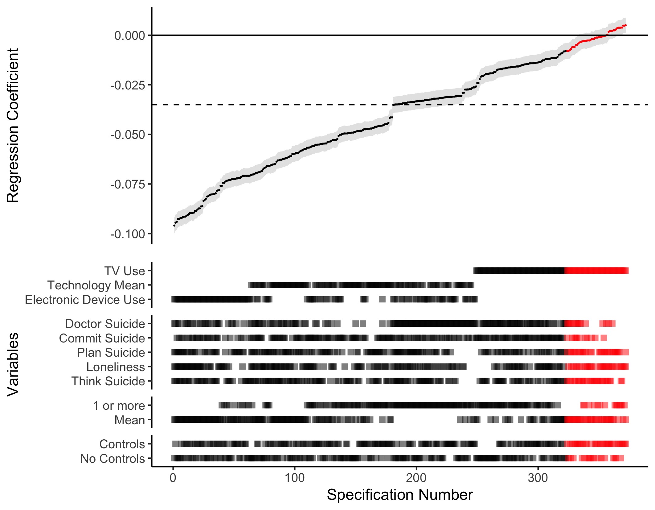
Figure 2.2: Results of Specification Curve Analysis of the Youth Risk and Behaviour Survey: Specification Curve Analysis showing the range of possible results for a simple cross-sectional regression of digital technology use on adolescent well-being. Each point on the x-axis represents a different combination of analytical decisions, which are displayed in the ‘dashboard’ at the bottom of the graph. The resulting standardised regression coefficient is shown at the top of the graph; the error bars visualise the standard error. Red represents non-significant outcomes, while black represents significant outcomes. To ease interpretation, the dotted line indicates the median standardised regression coefficient found in the Specification Curve Analysis: = -.035 (median partial = .001, median = 62,297, median standard error = .004)
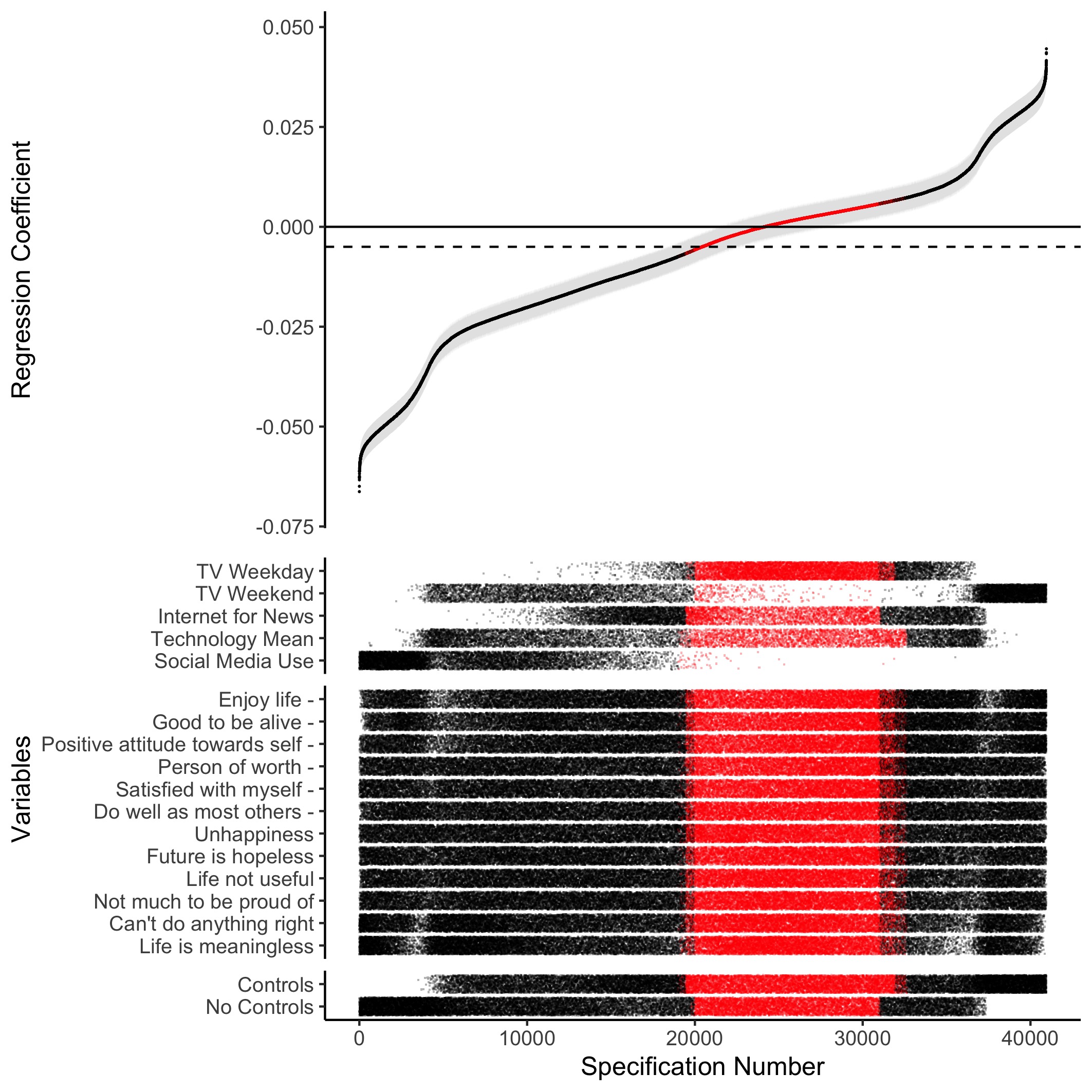
Figure 2.3: Results of Specification Curve Analysis of the Monitoring the Future study: Specification Curve Analysis showing the range of possible results for a simple cross-sectional regression of digital technology use on adolescent well-being. Each point on the x-axis represents a different combination of analytical decisions, which are displayed in the ‘dashboard’ at the bottom of the graph. The resulting standardised regression coefficient is shown at the top of the graph; the error bars visualise the standard error. Red represents non-significant outcomes, while black represents significant outcomes. To ease interpretation, the dotted line indicates the median standardised regression coefficient found in the Specification Curve Analysis: = -.005 (partial < .001, median = 78,267, median standard error = .003)
For the MTF data, a median standardised of -.005 was observed (median partial < .001, median n = 78,267, median standard error = .003), a value which fell into the non-significant range of the justifiable specifications (see Figure 2.3). This result was surprising, as MTF had the highest number of observations, making it difficult for even small associations to be flagged as non-significant using traditional thresholds (i.e., p < .05). In Figure 2.3, and my bootstrapping test, I do not include the few specifications of the participants that only filled in one well-being measure (to see the SCA of all participants, see Figure A.5). From Figure 2.3 it is again possible to discern that even controls of lower standard made the association either less negative or even positive (no controls: median = -.013, median partial < .001, median n = 117,560, median standard error = .003; controls: median = .001, median partial < .001, median n = 72,525, median standard error = .003). TV viewing on the weekend had a median positive association with well-being of = .008 (median partial = .001, median n = 115,738, median standard error = .003), while social media use had a median negative association with well-being of = -.031 (median partial = .001, median n = 102,963, median standard error = .003), though the effect was small suggesting that technology use operationalised in these terms accounts for less than 0.1% of the observed variability in well-being. Using the internet for news and TV viewing on a weekday showed mainly very small median associations, = -.002 (median partial < .001, median n = 115,580, median standard error = .003) and = .002 (median partial < .001, median n = 115,783, median standard error = .003) respectively. As previous studies have addressed the association between technology use and well-being using the same dataset (Twenge et al. 2017), I include Figure 2.4 which shows how these study’s specifications influence their reported results.
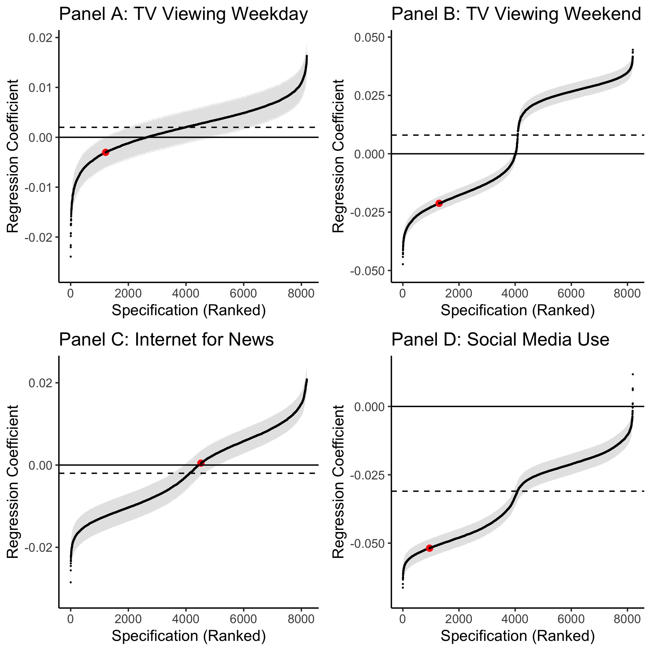
Figure 2.4: Each panel of this figure illustrates the range of possible results found using a SCA regressing a specific technology use variable onto well-being in the MTF dataset: Panel A examines TV viewing on a weekday, Panel B examines TV viewing on a weekend, Panel C examines using the internet to get news and Panel D examines social media use. The error bars represent the standard error and the dotted line shows the median standardised regression coefficient. I highlight in red the specifications chosen by Twenge and colleagues (2017) for their analysis of the MTF dataset. The researchers used a novel combination of measures from both well-being and self-esteem scales to create a well-being scale in their study, see also Figure 2.1. They correlated this measure with technology use measures (TV viewing, using the internet for news and social media use) and included either no controls or range of controls variables. We only show Twenge et al.’s results with no controls in this visualisation due to their chosen controls being difficult to reproduce computationally. We note that our results from implementing Twenge and colleague’s specification for TV viewing are not consonant with those reported in Twenge et al. (2017). For TV viewing on a weekday the specifications chosen in Twenge et al. (2017) were at the 15th percentile of effect sizes, for TV viewing on a weekday they were at the 16th percentile. For getting news over the internet, the chosen specifications were at the 55rd percentile and for social media use the chosen values were at the 12th percentile.
Figure 2.5: Results of Specification Curve Analysis of the Millennium Cohort Study: Specification Curve Analysis showing the range of possible results for a simple cross-sectional regression of digital technology use on adolescent well-being. Each point on the x-axis represents a different combination of analytical decisions, which are displayed in the ‘dashboard’ at the bottom of the graph. The resulting standardised regression coefficient is shown at the top of the graph; the error bars visualise the standard error. Red represents non-significant outcomes, while black represents significant outcomes. To ease interpretation, the dotted line indicates the median standardised regression coefficient found in the Specification Curve Analysis: = -.032 (partial = .004, median = 7,968, median standard error = .010)
Lastly, results from MCS, the highest quality dataset I examined, were interesting because the literature provided us with control variables based on extant theory (Parkes et al. 2013) and convergent data from adolescent and caregiver reports. In these data I found a median of technology use’s association with wellbeing of = -.032 (median partial = .004, median n = 7,968, median standard error = .010, see Figure 2.5). Across the board, if using well-being measures completed by the caregivers, the median association was less negative or more positive (median < .001, median partial = .003, median n = 7,893, median standard error = .010), while the opposite was in evidence when considering well-being measures completed by the adolescent (median = -.046, median partial = .008, median n = 8,857, median standard error =. 010). This pattern of shared covariation speaks to the idea that correlations between technology use and well-being might be rooted in common method variance, as one single informant fills out well-being and technology measures and the association might be driven by other common factors.
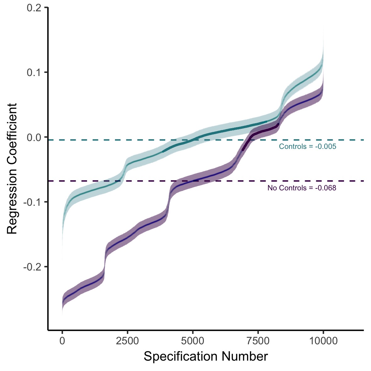
Figure 2.6: Results of Specification Curve Analysis of the Millennium Cohort Study split by whether control variables are included in the analysis or not: Specification Curve Analysis showing the range of possible results for a simple cross-sectional regression of digital technology use on adolescent well-being. Each specification number indicates a different combination of analytical decisions. The plot then shows the outcome of the corresponding analysis (standardised regression coefficient) either including control variables (teal, median standardised = -0.005, partial = .001, median = 6,566, median standard error = .011) or not including control variables (purple, median standardised = -0.068, partial = .005, median = 11,018, median standard error = .010). The bolded parts of the line indicate analyses that did not reach significance ( > 0.05). The median standardised regression coefficients for analyses including or not including control variables are shown using the dashed lines and the error bars visualise the standard error.
To further address the importance of control variables, I plot separate specification curves for MCS analyses with and without control variables (see Figure 2.6). The association for the uncorrected models had a median of -.068 (median partial = .005, median n = 11,018, median standard error = .010). In contrast, the corrected models only found a median of technology use regressed on wellbeing of -.005 (median partial = .001, median n = 6,566, median standard error = .011). Additional SCAs using only pre-specified questionnaires are presented in Figure A.1.
| Dataset | Observed Result | p value |
|---|---|---|
| YRBS | ||
| Median effect size | -0.040 | 0.00 |
| Share of results with dominant sign | 356 | 0.00 |
| Share of results with dominant sign & p <.05 | 323 | 0.00 |
| MTF | ||
| Median effect size | -0.007 | 0.00 |
| Share of results with dominant sign | 24149 | 0.00 |
| Share of results with dominant sign & p <.05 | 19636 | 0.00 |
| MCS | ||
| Median effect size | -0.045 | 0.00 |
| Share of results with dominant sign | 12481 | 0.00 |
| Share of results with dominant sign & p <.05 | 10857 | 0.00 |
2.3.3 III. Statistical Inferences
The SCAs showed that there is a small negative association between technology use and well-being, but it is not possible to make many statistical inferences because the specifications are not part of the same model and are therefore not independent. A bootstrapping technique was therefore used to run 500 SCA tests on resampled data, where it is known that the null hypothesis is true. Results presented in Table 2.3 indicate that the effects found were highly significant for all three datasets, and all three measures of significance included in my bootstrapped tests. For the three datasets, there was no SCA analysing bootstrapped samples which resulted in a larger median effect size than the median effect size of the original SCA ( = 0.00, original effect sizes: YRBS median = -.040, MTF median = -.007, MCS median = -.045). Furthermore, there was no bootstrapped SCA with more total or statistically significant specifications of the dominant sign than the original SCA (share of specifications with dominant sign p = 0.00; original number: YRBS = 356, MTF = 24,164, MCS = 12,481; share of statistically significant specifications with dominant sign p = 0.00; original number: YRBS = 323, MTF = 19,649, MCS = 10,857). This result provides evidence that digital technology use and adolescent well-being could be negatively related at above chance levels in my data.
2.3.4 IV. Comparison Specifications
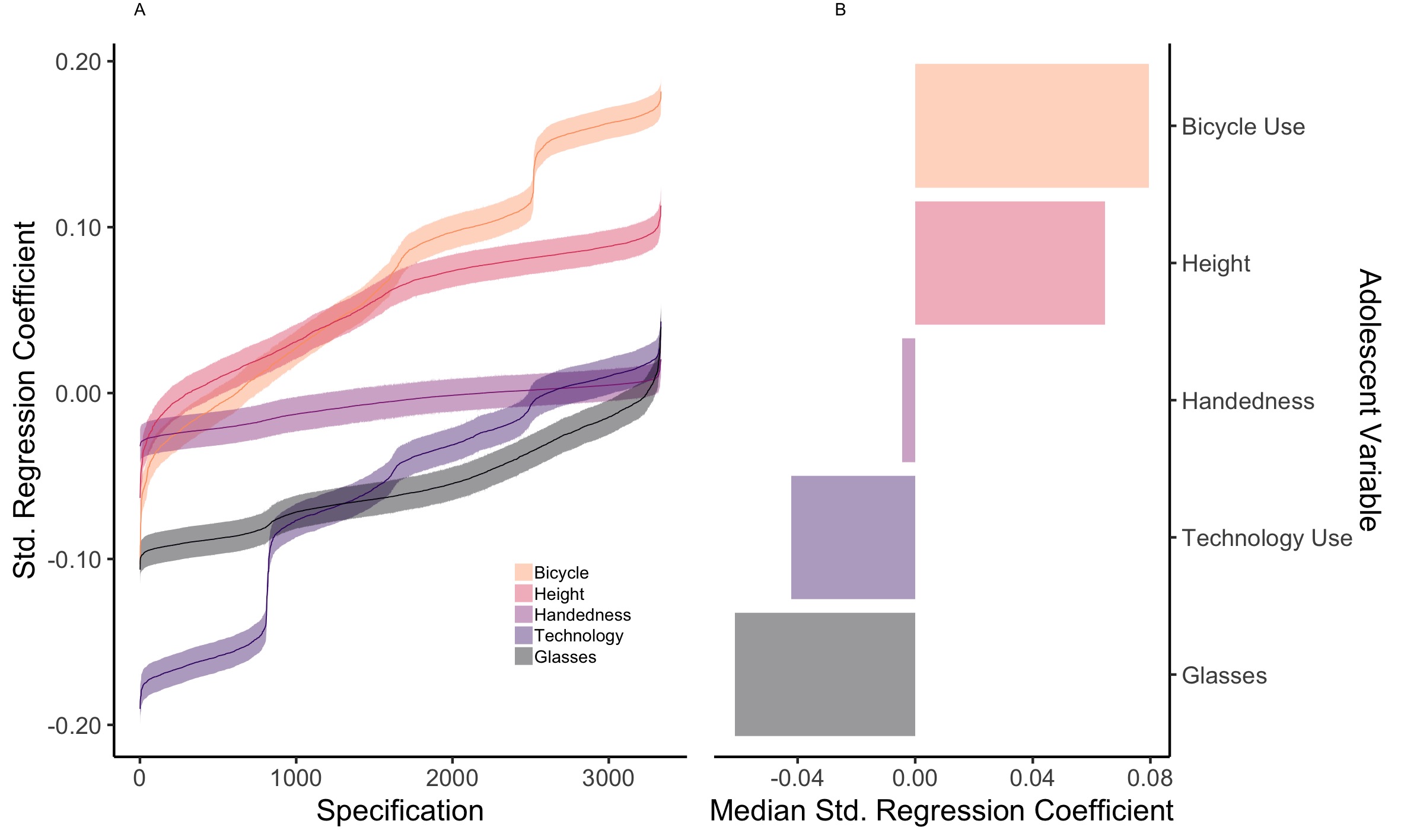
Figure 2.7: Visualisation of the comparison specifications for MCS hypothesised to have little or no influence on well-being: bicycle use, height, handedness and wearing glasses. This graph shows Specification Curve Analyses for both the variable of interest (mean technology use) and the comparison variables; It highlights the range of possible results of a simple cross-sectional regression of the variables of interest on adolescent well-being. Wearing glasses has the most negative association with adolescent well-being (black, median = -.061, median = 7,963, partial = .005, median standard error = .010), more negative than the association of technology use with well-being (purple, median = -.042, median = 7,964, partial = .002, median standard error = .010). Handedness (red/purple, median = -.004, median = 7,972, partial < 0.001, median standard error = .010), height of the adolescent (red, median = .065, median = 7,910, partial = .005, median standard error = .010) and whether the adolescent often rides a bicycle (yellow, median = .080, median = 7,974, partial = .007, median standard error = .010) have more positive associations with adolescent well-being than technology use does. Panel A shows how different analytical decisions (Specifications, shown on the x-axis) lead to different statistical outcomes (Standardised Regression Coefficient, shown on the y-axis). Each line represents a different variable of interest, the error bars represent the standard error. Panel B visualises the resulting Median Standardised Regression Coefficients for those Specification Curve Analyses linking the variables of interest with adolescent well-being.
To put the results of the SCAs into perspective with respect to the broader context of human behaviour as measured in these datasets, I compare specification curves for the mean of the technology use variables in each dataset to other associations that have been shown to relate, or are hypothesised not to relate, to adolescent mental health: binge drinking, smoking marijuana, being bullied, getting into fights, smoking cigarettes, being arrested, perceived weight, eating potatoes, having asthma, drinking milk, going to the movies, religion, listening to music, doing homework, cycling, height, wearing glasses, handedness, eating fruit, eating vegetables, getting enough sleep and eating breakfast. For results see Table 2.4 at the end of the chapter and Figures 2.7-2.10).
| Factor | Comparison Specifications | YRBS | MTF | MCS |
|---|---|---|---|---|
| Negative Factors | Binge drinking | 2.95x | 8.10x | 1.02x |
| Marijuana | 2.70x | 10.09x | 1.14x | |
| Bullying | 4.33x | – | 4.92x | |
| Getting into fights | 3.65x | 15.58x | – | |
| Cigarettes | – | 18.47x | – | |
| Being arrested | – | – | 0.96x | |
| Neutral Factors | Perceived weight | 1.02x | – | – |
| Potatoes | 0.86x | – | – | |
| Asthma | 1.34x | – | – | |
| Milk | 0.28x* | – | – | |
| Going to Movies | – | 11.51x* | – | |
| Religion | – | 16.29x* | – | |
| Music | – | 32.68x | – | |
| Homework | – | 3.57x* | – | |
| Cycling | – | – | 1.88x* | |
| Height | – | – | 1.53x* | |
| Glasses | – | – | 1.45x | |
| Handedness | – | – | 0.10x | |
| Positive Factors | Fruit | 0.11x | 9.49x* | 1.32x* |
| Vegetables | 0.27x | 20.63x* | 1.52x* | |
| Sleep | 3.06x* | 44.23x* | 1.65x* | |
| Breakfast | 2.37x* | 30.55x* | 3.32x* |
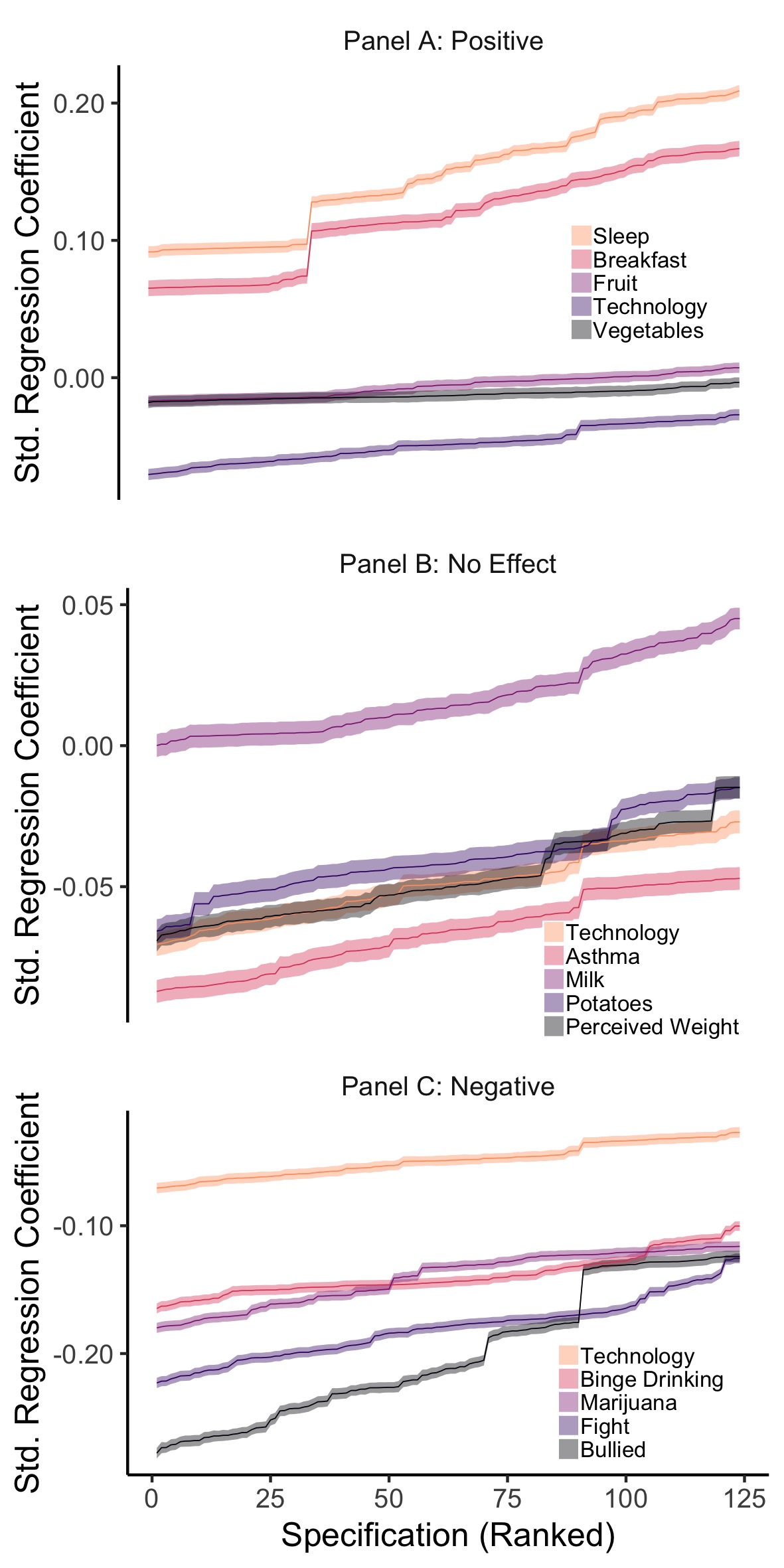
Figure 2.8: YRBS Comparison Specification Curves, split into three panels to compare the effect of technology use on wellbeing to other hypothesised positive (Panel A), neutral (Panel B) and negative factors (Panel C). The figure shows the results of 15 SCAs: illustrating the range of possible regression coefficients found when examining the association between well-being and other variables. The error bars represent the corresponding Standard Error.
For YRBS (Figure 2.8), the association of mean technology use with well-being (median = -.049, median n = 62,166, partial = .002, median standard error = .004) was exceeded by well-being’s association with being bullied (median = -.212, median n = 50,066, partial = .044, median standard error = .004), getting into fights (median = -.179, median n = 62,106, partial = .031, median standard error = .004), binge drinking (median = -.144, median n = 62,010, partial = .021, median standard error = .004), smoking marijuana (median = -.132, median n = 62,361, partial = .018, median standard error = .004), having asthma (median = -.066, median n = 60,863, partial = .004, median standard error = .004) and perceived weight (median = -.050, median n = 62,752, partial = .002, median standard error =.004). There is a smaller negative association for eating potatoes (median = -.042, median n = 61,912, partial = .002, median standard error = .004), eating vegetables (median = -.013, median n = 62,034, partial < .001, median standard error = .004) and eating fruit (median = -.005, median n = 62,436, partial < .001, median standard error = .004). There is a smaller positive association for drinking milk (median = .014, median n = 60,021, partial < .001, median standard error = .004). Lastly, there is a larger positive association for eating breakfast (median = .116, median n = 34,010, partial = .013, median standard error = .006) and getting enough sleep (median = .150, median n = 56,552, partial = .022, median standard error = .004).
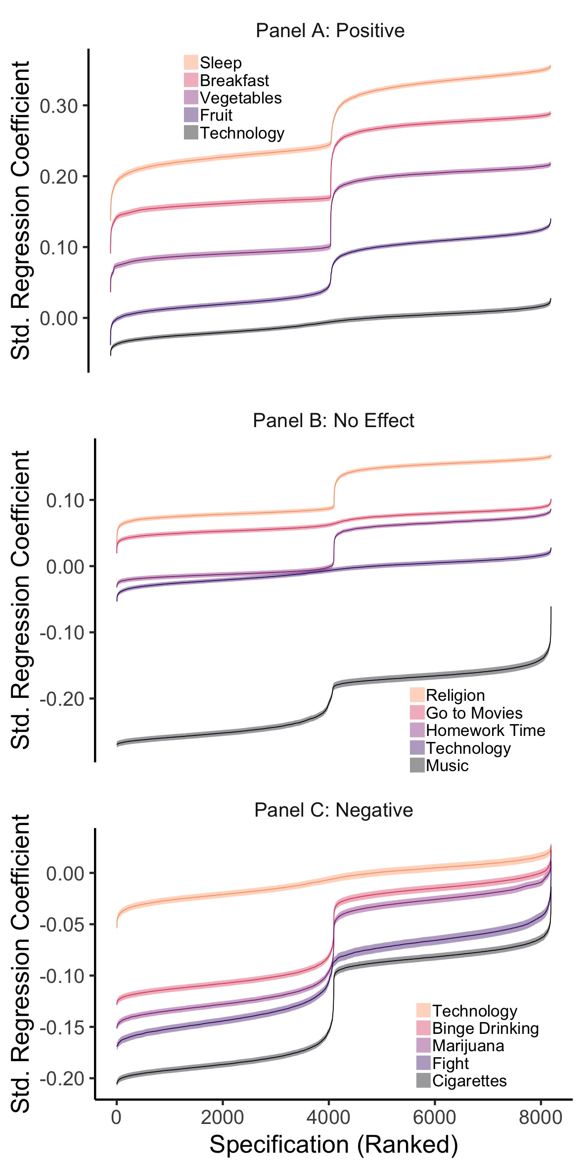
Figure 2.9: MTF Comparison Specification Curves, split into three panels to compare the effect of technology use on wellbeing to other hypothesised positive (Panel A), neutral (Panel B) and negative factors (Panel C). The figure shows the results of 15 SCAs: illustrating the range of possible regression coefficients found when examining the association between well-being and other variables. The error bars represent the corresponding Standard Error.
For the MTF (Figure 2.9), I compare the association of mean technology use with well-being (median = -.006, median n = 102,186, partial < .001, median standard error = .003) to the variables I hypothesised a priori to have no association: going to the movies (median = .064, median n = 115,943, partial = .005, median standard error = .003), time spent on homework (median = .020, median n = 115,225, partial = .001, median standard error = .003), attending religious services (median = .091, median n = 89,453, partial = .010, median standard error = .003) and listening to music (median = -.182, median n = 49,514, partial = .035, median standard error = .005) all had larger effects. I also examined those comparison variables I hypothesised to have a more positive association: eating breakfast (median = .170, median n = 62,330, partial = .034, median standard error = .004), eating fruit (median = .053, median n = 115,334, partial = .003, median standard error = .003), sleep (median = .246, median n = 61,903, partial = .070, median standard error = .004), and eating vegetables (median = .115, median n = 62,072, partial = .014, median standard error = .004). Lastly, I looked at those variables that I hypothesised to have a more negative association: binge drinking (median = -.045, median n = 107,994, partial = .002, median standard error = .003), fighting (median = -.087, median n = 62,683, partial = .008, median standard error = .004), smoking marijuana (median = -.056, median n = 113,611, partial = .003, median standard error = .003) and smoking cigarettes (median = -.103, median n = 113,424, partial = .012, median standard error = .003).
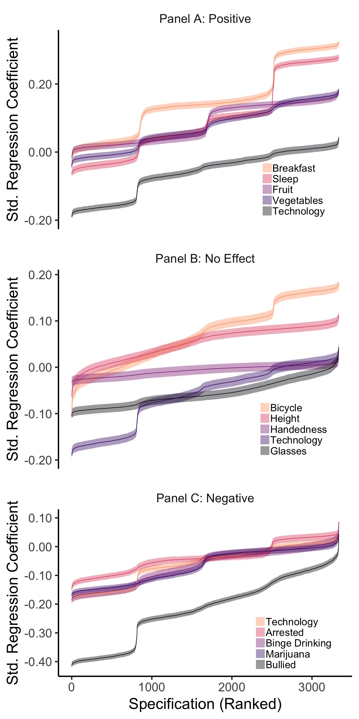
Figure 2.10: MCS Comparison Specification Curves, split into three panels to compare the effect of technology use on wellbeing to other hypothesised positive (Panel A), neutral (Panel B) and negative factors (Panel C). The figure shows the results of 15 SCAs: illustrating the range of possible regression coefficients found when examining the association between well-being and other variables. The error bars represent the corresponding Standard Error.
For MCS (Figure 2.10), mean technology use (median = -.042, median n = 7,964, partial = .002, median standard error = .010) was compared to amount of sleep (median = .070, median n = 7,954, partial = .005, median standard error = .010), eating fruit (median = .056, median n = 7,960, partial = .004, median standard error = .010), eating breakfast (median = .140, median n = 7,964, partial = .025, median standard error = .010) and eating vegetables (median = .064, median n = 7,949, partial = .005, median standard error = .010) that have a priori hypothesised positive associations; being arrested (median = -.041, median n = 7,908, partial = .002, median standard error = .011), being bullied (median = -.208, median n = 7,898, partial = .048, median standard error = .010), binge drinking (median = -.043, median n = 3,656, partial = .002, median standard error = .015) and smoking marijuana (median = -.048, median n = 7,903, partial = .003, median standard error = .010) that have a priori hypothesised negative associations; wearing glasses (median = -.061, median n = 7,963, partial = .005, median standard error = .010), being left-handed (median = -.004, median n = 7,972, partial < 0.001, median standard error = .010), bicycle use (median = .080, median n = 7,974, partial = .007, median standard error = .010) and height (median = .065, median n = 7,910, partial = .005, median standard error = .010) that have no a priori hypothesised associations (also see Figure 2.7).
2.4 Discussion
The possibility that adolescents’ digital technology use has a negative impact on psychological well-being is an important question worthy of rigorous empirical testing. While previous research in this area has equated findings derived from large-scale social data with empirical robustness, the present research highlights deep-seated problems associated with drawing strong inferences from such analyses. To provide a robust and transparent investigation of the association of digital technology use with adolescent well-being, I implemented Specification Curve Analysis (SCA) with comparison specifications using three large-scale datasets from the US and UK.
While I find that digital technology use has a small negative association with adolescent well-being, this finding is best understood in terms of other human behaviours captured in these large-scale social datasets. When viewed in the broader context of the data, it becomes clear that the outsized weight given to digital screen time in scientific and public discourse might not be merited on the basis of the available evidence. For example, in all three datasets the associations found for both smoking marijuana and bullying have larger negative associations with adolescent well-being (2.7x and 4.3x respectively for YRBS) than technology use does. Positive antecedents of well-being are equally illustrative; simple actions like getting enough sleep and regularly eating breakfast have much more positive associations with well-being than the average impact of technology use (ranging from 1.7x to 44.2x more positive in all datasets). Neutral factors provide perhaps the most useful context to judge technology engagement effects: the association of well-being with regularly eating potatoes was nearly as negative as the association with technology use (0.9x, YRBS) and wearing glasses was more negatively associated with well-being (1.5x, MCS).
With this in mind, the evidence simultaneously suggests technology effects might be statistically significant but so minimal that they hold little practical value. The nuanced picture these results provide are in line with previous psychological and epidemiological research suggesting the associations between digital screen time and adolescent outcomes are not as simple as many might think (Parkes et al. 2013; Przybylski and Weinstein 2017). This work therefore puts previous work that used the YRBS and MTF to highlight technology use as a potential culprit for decreasing adolescent well-being (Twenge et al. 2017) into perspective, showing the range of possible analytical results and comparison specifications. The finding that the association between digital technology use and well-being is much smaller than previously put forth has extensive implications for stakeholders and policy-makers considering monetary investments into decreasing technology use in order to increase adolescent well-being (Department of Health and Social Care 2018).
Importantly, the small negative associations diminish even further when proper and pre-specified control variables, or caretaker responses about adolescent well-being, are included in the analyses. This finding underlines the importance of considering high-quality control variables, a priori specification of effect sizes of interest, and a critical evaluation of the role that common method variance may play when mapping the effect of digital technology use on adolescent well-being (Ferguson 2009). It is not enough to rely on statistical power to improve scientific endeavour, large-scale social data analysis harbours its own challenges for statistical inference and scientific progress.
This investigation therefore highlights two intrinsic problems confronting behavioural scientists using large-scale social data. First, large numbers of ill-defined variables necessitate researcher flexibility, potentially exacerbating the garden of forking paths problem: for some datasets analysed there were more than a trillion different ways to operationalize a simple regression (Gelman and Loken 2014). Second, high numbers of observations render minutely small associations significant through the default NHST lens (Lakens and Evers 2014). With these challenges in mind, my approach, grounded in SCA and including comparison specifications presents a promising solution, so that behavioural scientists can build accurate and practically actionable representations of effects found in large-scale datasets. Overall, the findings place popular worries about the putative links between technology use and mental health indicators into context. They underscore the need for open and impartial reporting of small correlations derived from large-scale social data.
2.4.1 Limitations
My analyses, however, do not provide a definite answer to whether digital technology impacts adolescent well-being. Firstly, it is important to note that using most large-scale datasets one can only examine cross-sectional correlations links, and it is therefore unclear what is driving effects where present. I know very little about whether more technology use might cause lower well-being, whether lower well-being might cause more technology use or whether a third confounding factor underlies both (see Chapter 4). As I am examining something inherently complex, the likelihood of unaccounted factors affecting both technology use and wellbeing is high. It is therefore possible that the associations I document, and those that previous authors have documented, are spurious.
For the sake of simplicity and comparison, simple linear regressions were used in this study, overlooking the fact that the relationship of interest is probably more complex, non-linear, or hierarchical (Przybylski and Weinstein 2017). Many measures used were also of low quality, non-normal, heterogenous, or outdated, limiting the generalisability of the study’s inferences. As self-report digital technology measures are known to be noisy (Scharkow 2016), this could have also led to the association of technology use with well-being being diminished due to low-quality measurement (addressed in Chapter 3). Lastly, I used NHST to interpret significance, which is problematic when using such extensive data. To improve, partnerships between research councils and behavioural scientists to better measurement, and pre-registering of analyses plans, will be crucial.
2.5 Conclusion
Whether they are collected as part of multi-lab projects or research council funded cohort studies, large-scale social datasets are an increasingly important part of the research infrastructure available for psychologists wanting to study emergent technologies. On balance, I am optimistic these investments provide an invaluable tool for studying technology effects in adolescents. To realise this promise, I firmly believe researchers must ground their work and debate in open and robust practices. In the quest for high power, I caution scientists studying emergent technology effects to understand the intrinsic limitations of large-scale data and to implemented approaches that guard against researcher degrees of freedom. While preregistration might be implausible for analyses of open large-scale social data, methodologies like Specification Curve Analyses provide solutions that don’t only support robust statistical inferences, but also provide a comprehensive way to report the effects found for academia, policy and the public.
2.6 Acknowledgements
This chapter is based on the published work Orben, A., & Przybylski, A. K. (2019). The association between adolescent well-being and digital technology use. Nature Human Behaviour, 3(2), 173.
The National Institute on Drug Abuse provided funding for MTF conducted at the Survey Research Centre in the Institute for Social Research, University of Michigan; YRBS was collected by the Centres for Disease Control and Prevention; The Centre for Longitudinal Studies, UCL Institute of Education collected MCS and the UK Data Archive/UK Data Service provided the data; They bear no responsibility for its aggregation, analysis, or interpretation.
Thank you to U. Simonsohn, N. K. Reimer and N. Weinstein for their valuable input and J. M. Rohrer, U. Simonsohn, J. P. Simmons and L. D. Nelson for code provision. I also acknowledge the use of the University of Oxford Advanced Research Computing (ARC) facility in carrying out this research: http://dx.doi.org/10.5281/zenodo.22558.